Unlocking Financial Insights With Looker Studio and Cloud Run
Table of Contents
Are you curious about how much money you’re spending on coffees and fast food? There are countless apps out there that categorise your spending and offer valuable insights. Even banks are integrating this functionality into their banking apps! So why bother building your own solution? Here are three reasons why I built my transaction categorising pipeline: First, I’m interested in money in general and enjoy understanding trends in how I spend it. Second, I had my own way of categorising spending long before banks offered this feature for free, and I’m reluctant to change it! Lastly, there’s something satisfying about automating practical tasks, like categorising spending, making it a fun and interesting project! Whether any of these reasons resonate with you or you’re just curious about the process, read on to learn how to build your own personal transaction categorising pipeline in Google Cloud!
Looker Studio is a powerful free data visualisation tool.
1. Manual to Automatic
When I first started a full time job as a software engineer after university and received my first paycheck, I decided I’d keep track of what I spent in a spreadsheet. I’d set up a budget with categories like “groceries” and “petrol”, but as you might know if you keep a budget, it’s hard to stick to a budget if you don’t know what you’re spending money on.
In my spreadsheet, I set up some basic formulae that’d show me what I’d spent in each category for a month, and at the end of the month, I’d copy the data for the month to a different page where I had it laid out month by month in a very crude fashion. This process required me to periodically scroll through my transactions and assign a category manually, a laborious process which began to grow old.
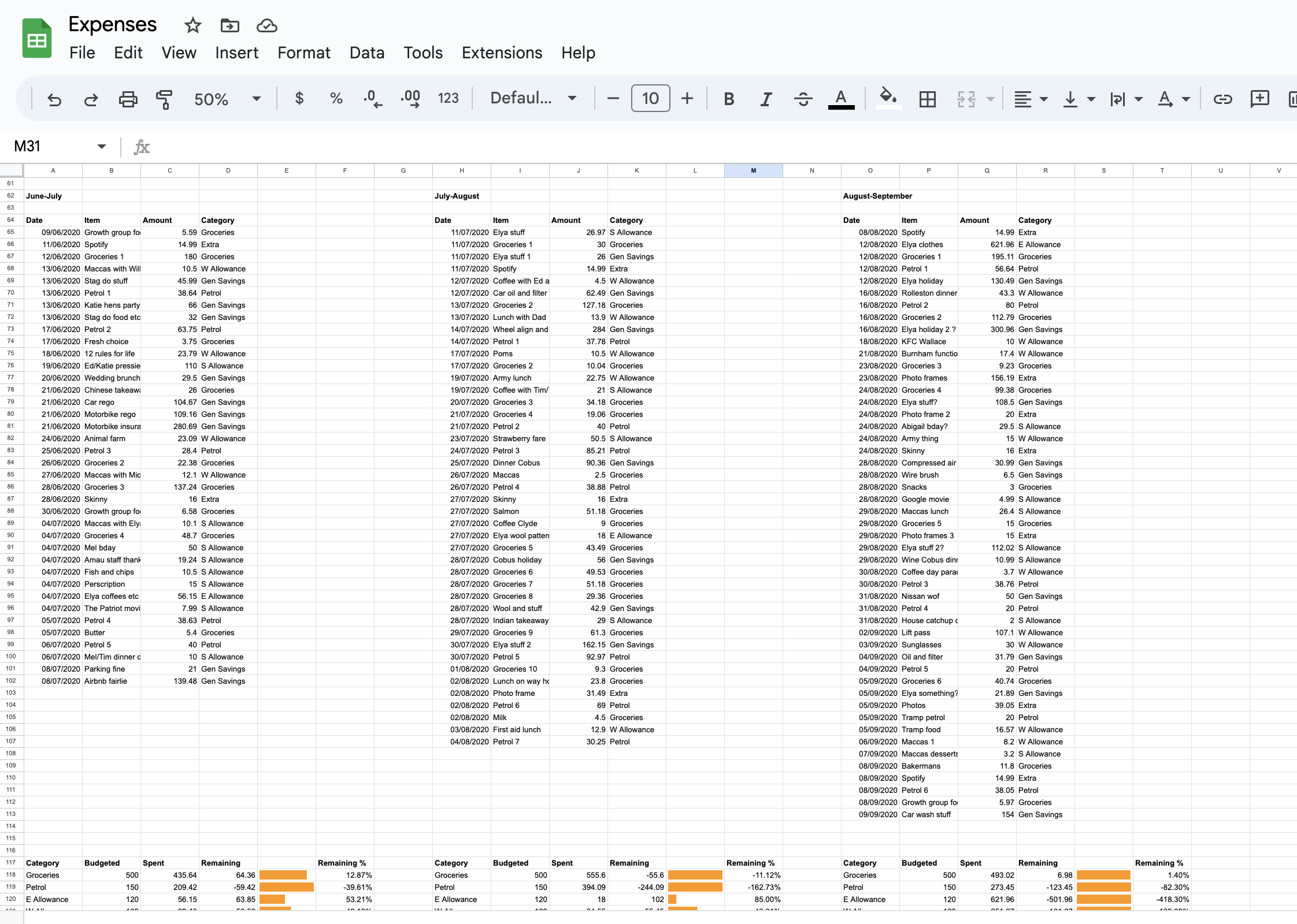
I quickly realised, although it looked fancy, this wasn’t a great way to store my data.
After a year or two of manually categorising in this way, I made a basic Python script which took a CSV of transactions from my account and assigned categories for some commonly occurring patterns. If the payee name contained “petrol” or “fuel” it was a safe bet that it’d be in the category petrol. If it contained the name of a few of the New Zealand supermarkets I visited such as “Countdown” or “New World”, it’d be groceries. The script would also filter out deposits as my budgeting was only concerned with my spending. This improved things a surprising amount, but it was still very manual.
Some time later and after much time spent manually trawling through transactions, I decided machine learning could be just what I was looking for to speed things up. The thought of a classifier which could accurately predict the majority of transactions and learn my categories as time went on was rather appealing. However, after searching for inspiration online I came across this article which convinced me that what I really needed was not actually machine learning, but rather, Elasticsearch. Elasticsearch is a search engine, optimised for searching text. I was aware of it as my work at the time used it for searching application logs, but I’d never considered it something I could use myself in a hobby project. I proceeded to download Elasticsearch and run it locally on a single node (Elasticsearch is designed to run on a cluster of nodes to make use of distributed processing). I loaded in my several year’s worth of categorised spending, and extended my Python script to use Elasticsearch’s fuzzy search which returned for a given transaction name, the most similar transaction name from my categorised data, as well as the category assigned to it. This worked fairly well, but as you may have guessed, it was like using a cannon to kill a mosquito. Plus it was a pain to have to start up Elasticsearch each time and remember to add the newly categorised transactions to the index.
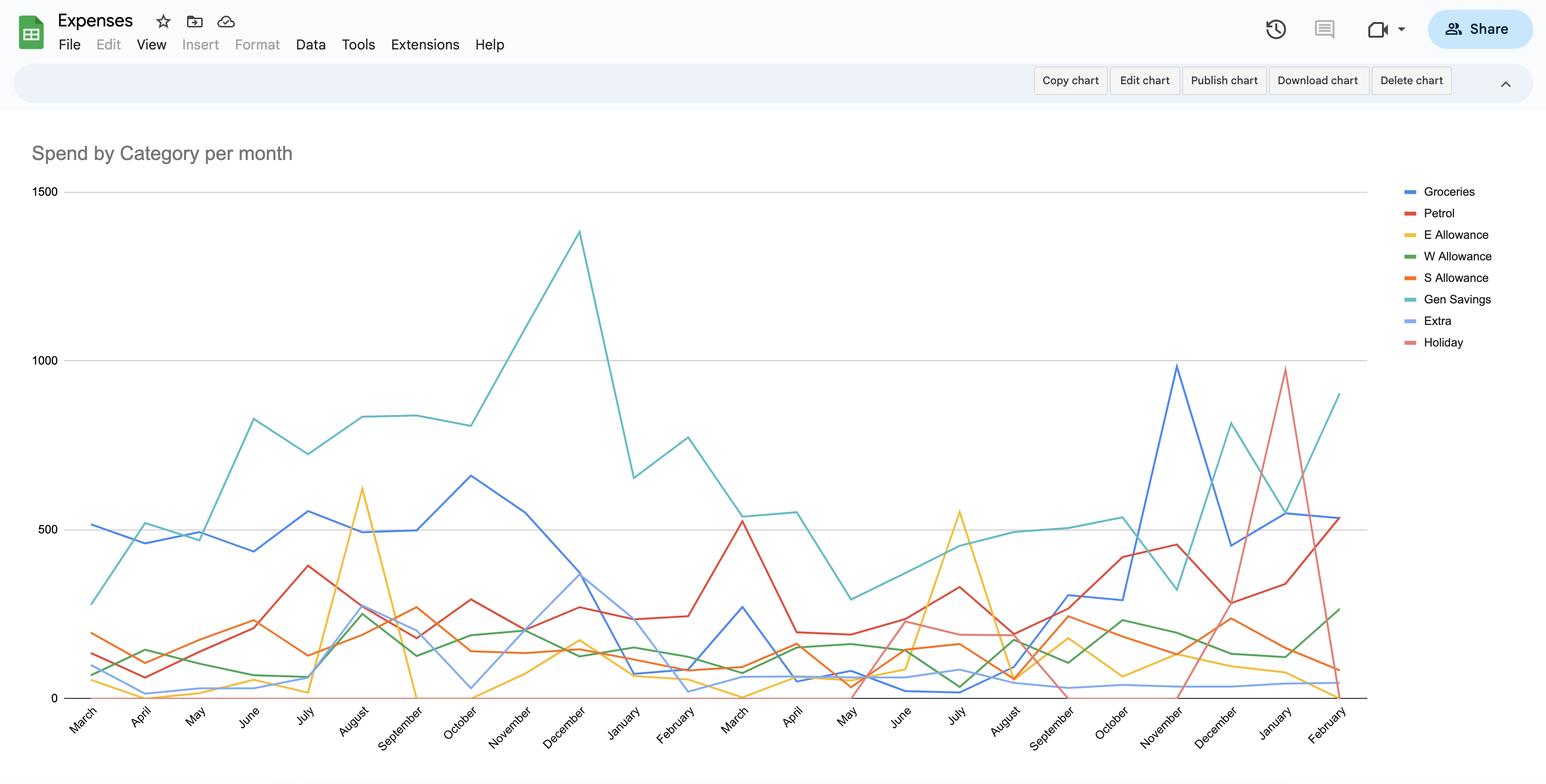
My spreadsheet produced some fairly unintuitive charts (to be fair, this was largely my fault) - nowhere near as powerful as Looker Studio which we’ll see shortly!
The next evolution was a return to the idea of using machine learning, possibly due to the hype around machine learning rather than any great conviction that it would work any better (spoiler: I should have heeded the advice from the previously mentioned article). I spent some time experimenting with training XGBoost and Random Forest models, attempting to make a classifier that would be able to predict categories from my dataset of about 1700 transactions. This may well have been a case of PEBCAK, but I was never able to get the accuracy passed the high 60%’s, despite several moments of triumph when I thought I’d trained a highly accurate mid 90% accuracy model only to realise I’d leaked test data into my training set.
The final iteration of my “automatic” categorising was a return to Elasticsearch’s fuzzy search, but instead of spinning up Elasticsearch each time I needed to categorise, I wrote a script which used the same algorithm that Elasticsearch uses without the Elasticsearch - the Levenshtein distance. The Levenshtein distance is the number of edits done to a string in order to match it to another. For example the Levenshtein distance between “cat” and “hat” is one because change “c” to an “h” and you get “hat”. This is a measure of how similar text is, and is relatively simple to implement. I admit I did ask ChatGPT to give me an implementation which worked out of the box, but I imagine there are plenty of Python implementations online.
The accuracy of this algorithm was around 75% which I was pretty happy with and after a few optimisations such as grouping together identical payee names to reduce the number of strings to compare (but still referring to the count of each unique payee), it performed categorisation of a month of transactions in a few seconds. If my dataset contained hundreds of thousands or millions of transactions, Elasticsearch might have been a more suitable option, but it was vastly overkill for my very small amount of data. At this stage my workflow looked something like:
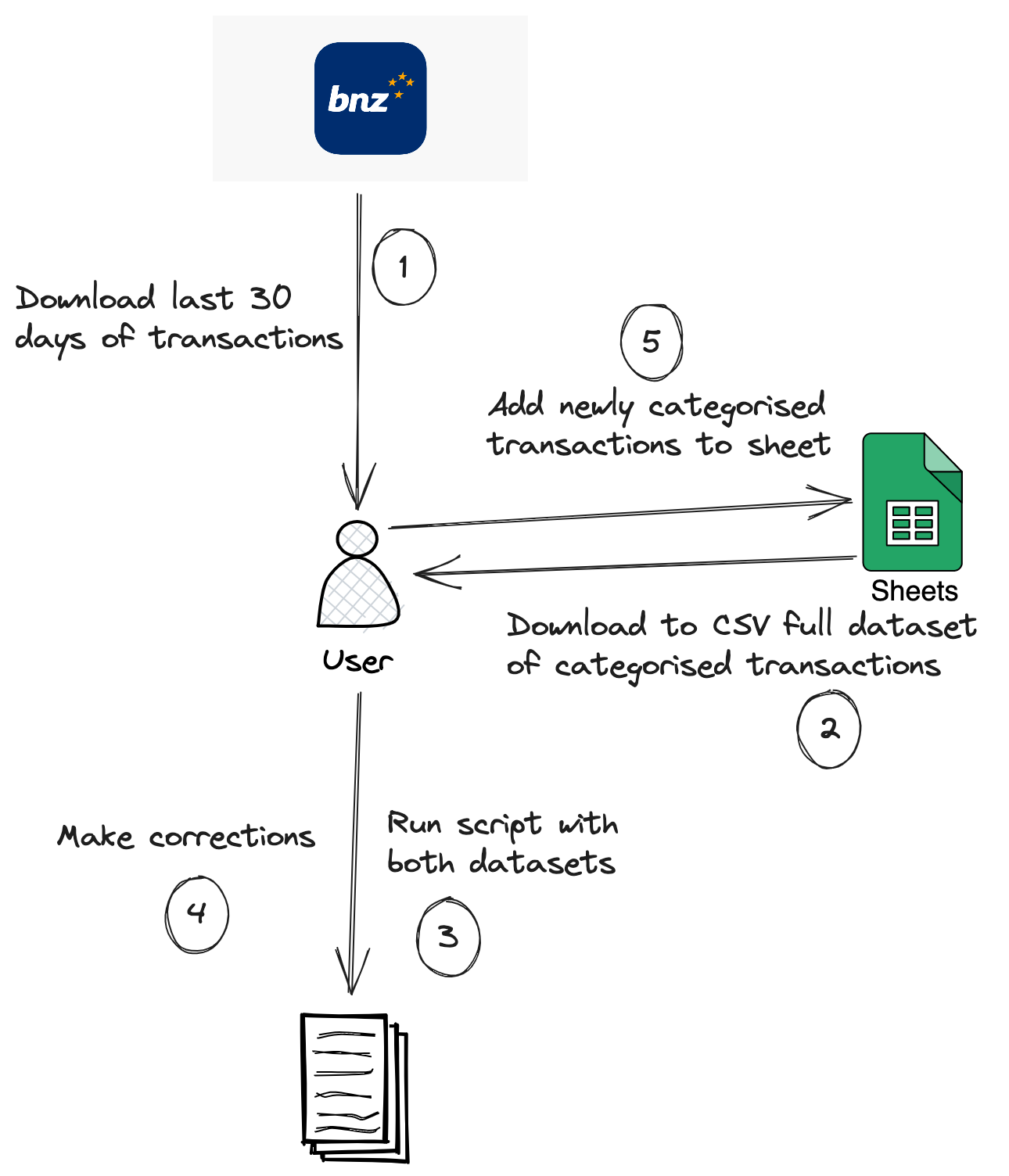
Still a lot of manual steps.
2. The Script Itself
The script I use is very much tailored to my particular bank which is Bank of New Zealand (BNZ) and I am quite certain it likely will not work with transactions from other banks, but it shouldn’t be too difficult to adapt. I imagine other banks have a similar name of a “Payee” for example, and it is simply a matter of modifying the code which loads the transactions into dataclass that needs tweaking to massage it into the correct form.
Helper functions
The original code for the Levenshtein distance generated by ChatGPT had variable names like “s” instead of “source_string” so for the reader’s benefit (and my own), I prompted ChatGPT to rewrite it with sensible variable names which it did.
from collections import Counter
from data_classes import TransactionOriginal, KnownPayee
from typing import List

def levenshtein_distance(source_string: str, target_string: str) -> int:
    """
    Computes the Levenshtein distance between two strings (written by ChatGPT).
    """
    source_len = len(source_string)
    target_len = len(target_string)

    # Create a matrix to store the distances between all possible pairs of substrings
    distance_matrix = [[0] * (target_len + 1) for _ in range(source_len + 1)]

    # Initialize the first row and column of the matrix
    for i in range(source_len + 1):
        distance_matrix[i][0] = i
    for j in range(target_len + 1):
        distance_matrix[0][j] = j

    # Fill in the matrix
    for j in range(1, target_len + 1):
        for i in range(1, source_len + 1):
            if source_string[i - 1] == target_string[j - 1]:
                substitution_cost = 0
            else:
                substitution_cost = 1
            distance_matrix[i][j] = min(distance_matrix[i - 1][j] + 1,  # Deletion
                                        distance_matrix[i][j - 1] + 1,  # Insertion
                                        distance_matrix[i - 1][j - 1] + substitution_cost)  # Substitution

    # The final element of the matrix is the Levenshtein distance between the strings
    return distance_matrix[source_len][target_len]
The Levenshtein distance simply calculates the distance between strings, and I still needed to be able to use it to find the most similar payee. The following (rather misleadingly named) function does this.
def closest_string(transactions: List[KnownPayee], target_transaction: TransactionOriginal, known_categories: dict, threshold: int=100) -> str:
    """
    Returns the value associated with the "Category" key in the dictionary from `strings` that has the smallest
    Levenshtein distance to the value associated with the "Payee" key in `target_dict`.
    If the closest distance is greater than `threshold`, returns "Unknown" (written by ChatGPT).
    """
    target_payee = target_transaction.payee

    known_categories_for_target = known_categories.get(target_payee)
    if known_categories_for_target is not None:
        highest_category = max(known_categories_for_target, key=known_categories_for_target.get)
        return highest_category

    closest_distance = float('inf')
    closest_rows = []
    for row in transactions:
        payee = row.payee
        distance = levenshtein_distance(payee, target_payee)
        if distance < closest_distance:
            closest_rows = [row.category]
            closest_distance = distance
        elif distance == closest_distance:
            closest_rows.append(row.category)
    if closest_distance <= threshold:
        # Pick the category of the most frequently occurring of the most similar payees
        return Counter(closest_rows).most_common(1)[0][0]
    else:
        return "Unknown"
Main script
The main script begins with a few imports:
import datetime
import math
from typing import List
from data_classes import TransactionOriginal, CategorisedTransaction, KnownPayee
from custom_category_assigner import closest_string
Followed by a few more helper functions:
def date_string_is_newer_than(date_to_compare: datetime.date, latest_record_date: datetime.date) -> bool:
    return date_to_compare > latest_record_date


def transaction_not_in_list(transaction: TransactionOriginal, seen_transactions: List[KnownPayee]) -> bool:
    return not any(
            item.payee == transaction.payee and math.isclose(float(item.amount), float(transaction.amount) * -1)
            for item in seen_transactions
    )


def is_relevant_transaction(row: TransactionOriginal) -> bool:
    # ignore transfers between funds and deposits
    return row.amount < 0 and row.reference != "INTERNET XFR" and row.tran_type != "FT"


def is_transaction_from_credit_card(row: TransactionOriginal) -> bool:
    return row.tran_type == "BP" and row.reference != "" and row.payee.lower() == "elya cox"


def count_categories_per_payee(transactions: List[KnownPayee]) -> dict:
    payee_categories = {}
    for transaction in transactions:
        payee = transaction.payee
        category = transaction.category
        if payee not in payee_categories:
            payee_categories[payee] = {}
        if category not in payee_categories[payee]:
            payee_categories[payee][category] = 0
        payee_categories[payee][category] += 1
    return payee_categories
The main function I’ve given the enlightening name of “predict_categories”. It could probably do with a good tidy up:
def predict_categories(categorised_dataset: List[KnownPayee], data_to_assign_categories: List[TransactionOriginal],
                       known_categories_and_counts: dict) -> List[CategorisedTransaction]:
    if len(categorised_dataset) == 0:
        return []
In order for the script to be able to handle a CSV downloaded from the banking website which contained transactions I’ve already categorised, I need to be able to filter out these already seen transactions. I do this by finding the most recent date amongst the categorised transactions dataset, getting the categorised transactions on this date, and comparing the list of transactions to be categorised. Are you sick of reading the words “categorised” and “transactions” yet?!
    most_recent_date = max(categorised_dataset, key=lambda x: x.date).date
    categorised_transactions_on_most_recent_date = [item for item in categorised_dataset if
                                                    item.date == most_recent_date]
    # TODO format this better
    filtered_transactions: List[TransactionOriginal] = [
        transaction for transaction in data_to_assign_categories
        if date_string_is_newer_than(transaction.date, most_recent_date) or (transaction.date == most_recent_date and transaction_not_in_list(transaction,
                                                                                categorised_transactions_on_most_recent_date))
    ]
    print(f"Found {len(filtered_transactions)} new transactions")
I then filter out various transactions using the helper functions from above. Things like deposits and transfers between my own accounts are not used so are discarded.
    filtered_data_to_categorise: List[TransactionOriginal] = [row for row in filtered_transactions if is_relevant_transaction(row)]

    if len(filtered_data_to_categorise) == 0:
        print("No rows found to assign categories to")
        return []

    rows: List[CategorisedTransaction] = []
    for row in filtered_data_to_categorise:
        payee = row.payee
A special case which is handled is my wife’s credit card. For transactions to pay off purchases on her credit card, she puts the name of the item in the reference. I extract this reference and replace the payee name with it. Otherwise, all transactions using her credit card would be assigned the same category because they’d be whatever’s most commonly associated with the payee which is her maiden name “Elya Cox”.
        if is_transaction_from_credit_card(row):
            payee = row.reference

        amount = row.amount * -1
        category = closest_string(categorised_dataset, row, known_categories_and_counts)
        categorised_row = CategorisedTransaction(date=row.date,
                                                 payee=payee,
                                                 amount=amount,
                                                 category=category,
                                                 particulars=row.particulars,
                                                 code=row.code,
                                                 reference=row.reference)
        rows.append(categorised_row)
    return rows
This is all bundled together in a function called “process”:
def process(data_to_categorise: List[TransactionOriginal], categorised_data: List[KnownPayee]) -> List[CategorisedTransaction]:
    known_categories = count_categories_per_payee(categorised_data)
    predicted_data = predict_categories(categorised_data, data_to_categorise, known_categories)

    return predicted_data
3. Deploying the Script with Cloud Run
For a time I did simply run this script manually and add the results to my spreadsheet as in previous iterations. After working with Google Cloud Platform (GCP) however, and realising that it has a rather generous free tier, I set out to host my workflow in the cloud. The general outline of this workflow looked like the following:
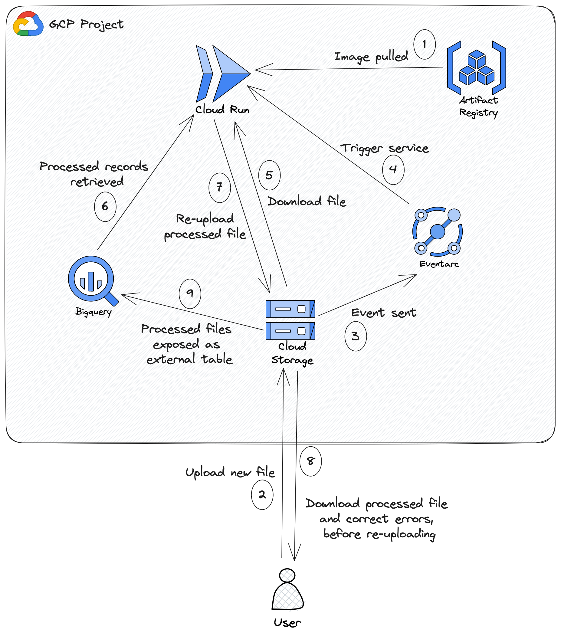
The categorising script now ran in the clouds!
Because at the time of writing, BNZ (and banks in New Zealand in general) do not yet support Open Banking APIs, I still need to do the painfully manual step of downloading a CSV of my account from the bank website. This involves logging in with two-factor authentication and my access number which I can never remember despite doing this fairly regularly - an all round annoying process. Once BNZ supports an API allowing me to programmatically retrieve transactions from my account, I’ll use Cloud Scheduler to periodically trigger a Cloud Run job to automate this manual step.
Therefore, the process begins again with me downloading my CSV, but this time I deposit the CSV into a directory called to_process in a Google Cloud Storage bucket. A storage notification notifies Eventarc (a GCP service allowing the delivery
of events in response to all sorts of GCP actions) which triggers a Cloud Run service. I’m aware that a Cloud Run job could be more appropriate than a service, but at the time of making this, Cloud Run jobs were still quite new, and so I went with a
service which seem easy and well documented. This service downloads already categorised data by querying interested columns from a BigQuery (GCP’s data warehouse) external table which exposes data in the processed directory of the same bucket. Along with this and the file that was uploaded to the
to_process directory, the service runs my categorising script and re-uploads the categorised file to a final directory called staging. I then download this, fix up any errors, and at last upload it to the processed directory where it’s queryable through the
BigQuery external table.
This may seem still like a number of steps, but it really boils down to:
- Get the file from the bank website.
- Upload it to the bucket.
- Download the categorised file.
- Make corrections.
- Upload it again.
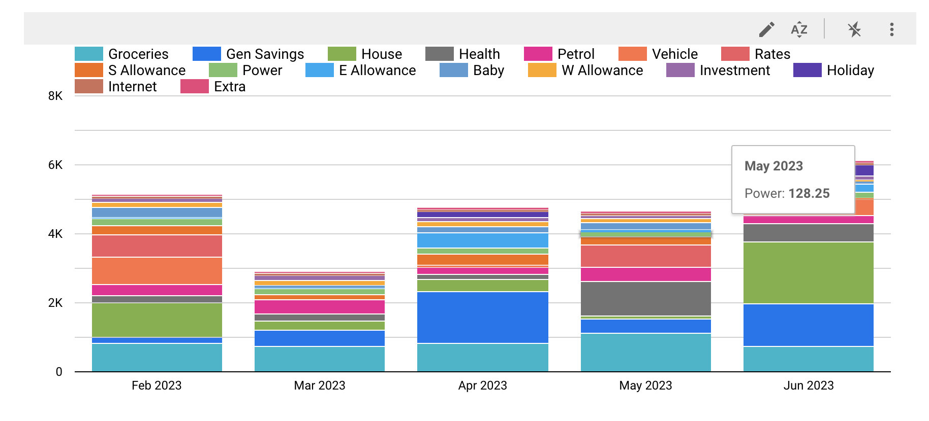
The BigQuery external table is connected to a Looker Studio dashboard which provides fast and easy insights into the data. For example, my dashboard (from which a monthly report is sent to my wife and I) shows our total spending month by month over time, allowing us to see if our spending is trending upwards. It also shows a visualisation of the breakdown of categories in each month. Clicking on a category in a particular month filters a table containing items in that category in that month. Clicking on a category filters the table to show items in that category for all the months in the visualisation.
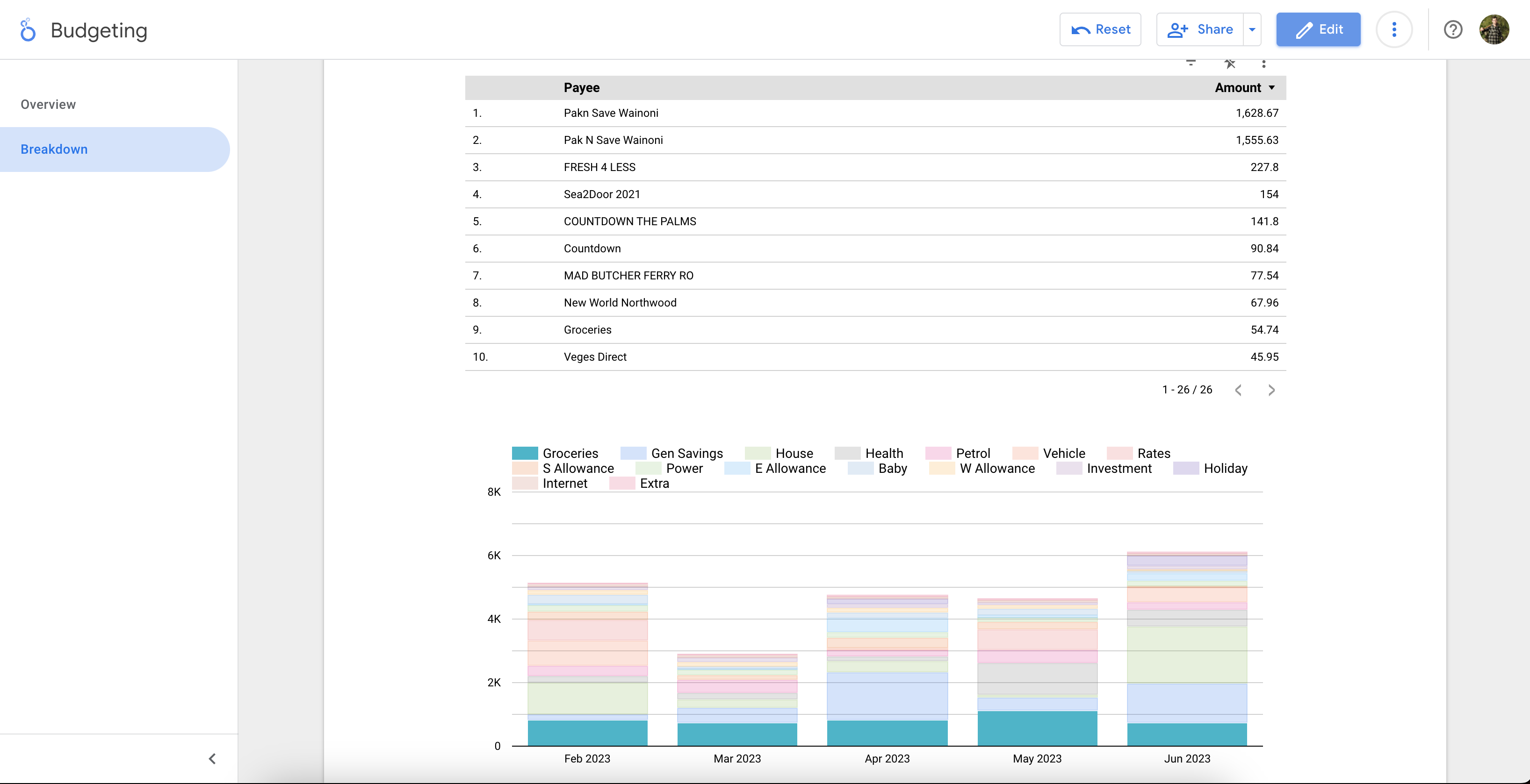
In this screenshot, I’m filtering by the grocery category which shows me in the table how much we’ve spent on each payee classified as groceries over the last 5 months.
My wife and I regularly consult this Looker Studio report and use it to decide on modifications to budgets. Say I receive a salary increase, and we have some more income to distribute. Having the data in this form provides us with the insight to determine which areas need an increase in budget and how much can go to savings or the mortgage. Without it, it’d be easy for us to fritter it away on things which don’t advance us towards our financial goals.
4. Infrastructure as Code
The pipeline which I’ve just described can certainly be created “click-ops” style by creating the various resources in the GCP UI (Cloud Console). To make it easier to keep track of changes and to be able to easily reproduce it, I’ve used Terraform (infrastructure as code tool)
to define my resources. If I needed to set up this pipeline for a friend or family member for example, it’d be as simple as creating a GCP project, enabling a few APIs and running terraform apply. To create this Terraform, I set up my repository with the following
Terraform files:
terraform
├── bigquery.tf
├── gcs.tf
├── main.tf
├── provider.tf
├── terraform.tfvars
├── variables.tf
I won’t go into detail on all the files (be sure to check out the repository linked at the end for the full code), but let’s look at a few.
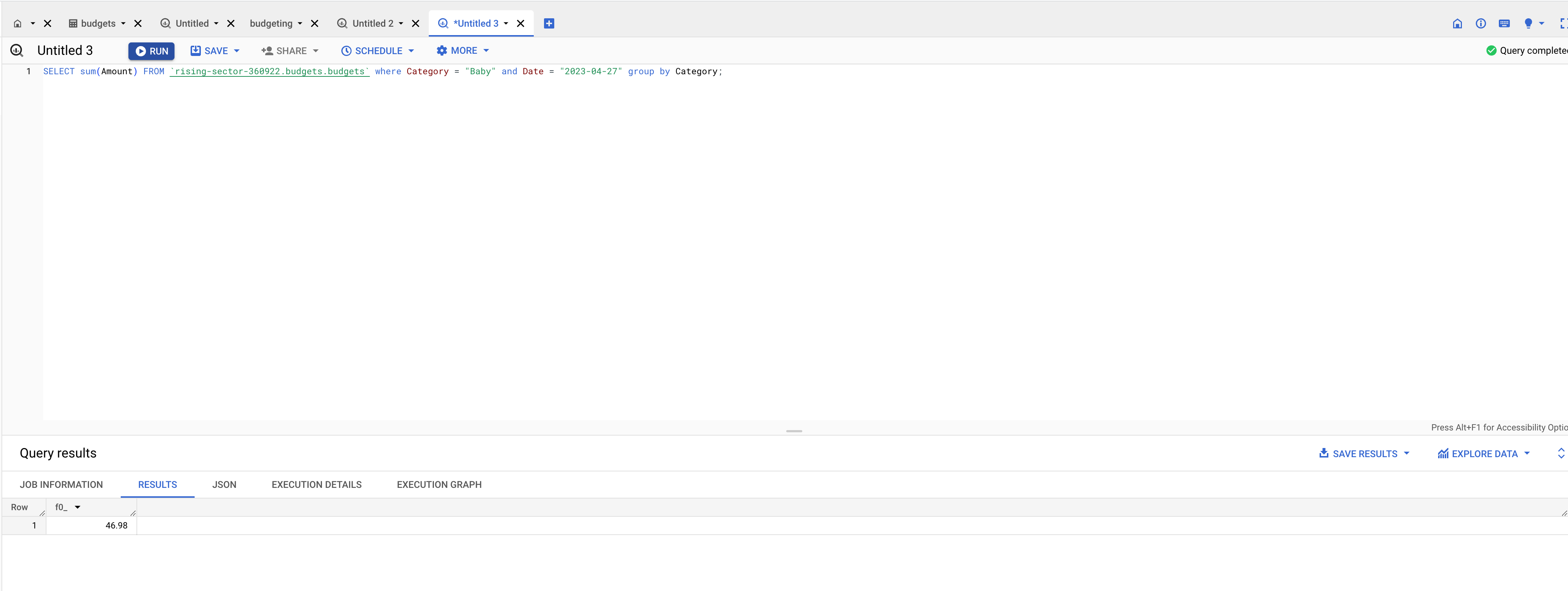
Besides Looker Studio, BigQuery can be used to query the data directly.
bigquery.tf
This tf file contains a BigQuery dataset and BigQuery external table. The external table lives in the dataset and points at a path in the Google Cloud Storage (GCS) bucket.
resource "google_bigquery_dataset" "budgets_dataset" {
  dataset_id    = var.bq_dataset
  friendly_name = var.bq_dataset
  description   = "Budgeting data"
  location      = var.location
}


resource "google_bigquery_table" "budget_external_table" {
  dataset_id = google_bigquery_dataset.budgets_dataset.dataset_id
  table_id   = var.bq_table
  deletion_protection=false

  external_data_configuration {
    autodetect    = false
    source_format = "CSV"

    csv_options {
      skip_leading_rows = 1
      quote             = ""
      field_delimiter   = ","
    }

    source_uris = [
      "gs://${google_storage_bucket.budget_data_bucket.name}${var.budget_files_path}/*.csv"
    ]

    schema = <<EOF
      [
        {
          "name": "Date",
          "type": "DATE",
          "mode": "REQUIRED"
        },
        {
          "name": "Payee",
          "type": "STRING",
          "mode": "REQUIRED"
        },
        {
          "name": "Amount",
          "type": "FLOAT",
          "mode": "REQUIRED"
        },
        {
          "name": "Category",
          "type": "STRING",
          "mode": "REQUIRED"
        },
        {
          "name": "Particulars",
          "type": "STRING",
          "mode": "NULLABLE"
        },
        {
          "name": "Code",
          "type": "STRING",
          "mode": "NULLABLE"
        },
        {
          "name": "Reference",
          "type": "STRING",
          "mode": "NULLABLE"
        }
      ]
      EOF
  }
}
gcs.tf
The gcs.tf file contains the GCS bucket and a reference to the GCS service agent (special Google managed service account for Cloud Storage) using the Terraform data source.
data "google_storage_project_service_account" "gcs_account" {
}

resource "google_storage_bucket" "budget_data_bucket" {
  name                     = var.budget_bucket
  location                 = var.location
  project                  = var.project_id
  public_access_prevention = "enforced"
}
main.tf
The main terraform file contains the Cloud Run service and Eventarc trigger, as well as a service account and some IAM bindings. The image tag for the Cloud Run service is configured as a variable so that it can be easily
updated to force the deployment of a new version of the service. In my repository, on a merge to the master/main branch, a GitHub action performs a Docker build and push if changes to the Python script are detected. It then updates the terraform.tfvars file
overwriting the existing value of the image tag variable. It then does a terraform apply which deploys a new version of the Cloud Run service with the changes to the script. I intend on covering this GitHub action in a separate post!
data "google_project" "project" {
  project_id = var.project_id
}

resource "google_service_account" "cloud_run_sa" {
  account_id = "budget-service"
  project = var.project_id
}

resource "google_cloud_run_v2_service" "budget" {
  name     = "budget-categorise"
  location = var.location
  ingress  = "INGRESS_TRAFFIC_INTERNAL_ONLY"

  template {
    service_account = google_service_account.cloud_run_sa.email

    scaling {
      max_instance_count = 1
    }

    containers {
      image = "${var.location}-docker.pkg.dev/${var.project_id}/budget-artifact-registry/category-assigner:${var.image_tag}"

      env {
        name  = "project_id"
        value = var.project_id
      }

      env {
        name  = "bq_dataset"
        value = var.bq_dataset
      }

      env {
        name  = "bq_table"
        value = var.bq_table
      }
    }
  }
}

# Create a GCS trigger
resource "google_eventarc_trigger" "trigger_bucket" {
  name     = "trigger-bucket"
  location = google_cloud_run_v2_service.budget.location

  matching_criteria {
    attribute = "type"
    value     = "google.cloud.storage.object.v1.finalized"
  }

  matching_criteria {
    attribute = "bucket"
    value     = google_storage_bucket.budget_data_bucket.name
  }

  destination {
    cloud_run_service {
      service = google_cloud_run_v2_service.budget.name
      region  = google_cloud_run_v2_service.budget.location
      path    = "/"
    }
  }

  service_account = google_service_account.cloud_run_sa.email

  depends_on = [google_project_iam_member.gcs_pubsub_member]
}

resource "google_project_iam_member" "gcs_pubsub_member" {
  project = var.project_id
  member  = "serviceAccount:${data.google_storage_project_service_account.gcs_account.email_address}"
  role    = "roles/pubsub.publisher"
}

resource "google_project_iam_member" "event_receiver_member" {
  project = var.project_id
  member = "serviceAccount:${google_service_account.cloud_run_sa.email}"
  role = "roles/eventarc.eventReceiver"
}
5. Closing Thoughts
Everyone has a different opinion on budgeting and managing finances. To me, the most crucial aspect is understanding how your money is spent. While banking apps or budgeting tools can offer some insights, why not take complete control of your financial data? With Cloud Run and Looker Studio, you have the power to deploy your budgeting solution for free, tailor it to your needs, and access valuable insights like never before. So, why wait? Check out the code here and start leveling up your budgeting today!