Building a Low Cost ML Pipeline in Google Cloud
One thing I really enjoy doing in my spare time is DIY and minor house renovations. In the two years of owning our first home, I’ve carried out weekend improvements from replacing curtain rails to re-leveling the lawn. Whether this passion for home maintenance is due to the New Zealand “Do It Yourself” culture or my desire to avoid spending money, I will leave it as an exercise for the reader to decide. Something that is certain however, is I struggle to see DIY projects to completion. There are a number of jobs around the house 95% done which have become de-prioritised and put off for another day. It’s difficult to maintain motivation when some other interesting task pops up. It’s much the same with personal software projects - Machine Learning (ML) ones in particular. Exploring some data in a notebook and getting a half decent model trained is the fun part; getting that model into production and serving predictions is a whole different story. There are plenty of platforms which make this much simpler (Vertex AI for example), but they inevitably cost money for the convenience, and as we’ve already established, that’s not hugely attractive to me. Driven by my frugal mindset, I embarked on a mission to build an ML pipeline for a house price prediction idea in Google Cloud Platform (GCP) from scratch. Join me as we dive into the journey of building this ML pipeline within GCP’s free tier, from inception to production.
If you’d like to skip ahead and see the finished product, visit the website House Pricer.
1 The Idea
House prices have been something that’s interested me for a long time. While enduring the roller coaster of house hunting as first home buyers, our weekends were filled with open homes and we began to feel an instinct towards what a house was worth based on features such as location, condition, size of the house and section. We’d consider the estimate from websites like Homes and OneRoof also, but at this time (close to the peak of prices post-Covid) house prices had increased quickly and as a rough rule we’d add $100k to the estimate these websites gave.
While I’m not a data scientist, I’ve worked on machine learning pipelines and dabbled with machine learning projects for interest. I was curious as to how difficult it’d be to train a machine learning model to predict prices better and with more accuracy than the likes of Homes and OneRoof. After managing to get hold of property sale data for Christchurch City and address data from Land Information New Zealand (LINZ), I set about experimenting in a notebook exploring the data and trialing different machine learning frameworks to see which gave the best results. It didn’t take too long to train a model which performed pretty well (predicting within around 5% of the actual prices as a median). The problem of course with this is most of the large property estimate websites don’t make it clear how accurate their predictions are so it was difficult to know whether this figure was good or bad. Only Homes, from what I could see, publish statistics on their estimate’s accuracy which I was able to use as a baseline.
Now that I had a model trained, the next step was to productionise it which meant building a pipeline so that new data could be acquired regularly, the data could be processed and combined into what the model expects, the model trained, and predictions made for houses all without any manual work on my part. The next section discusses what this eventually looked like.
2 The Design
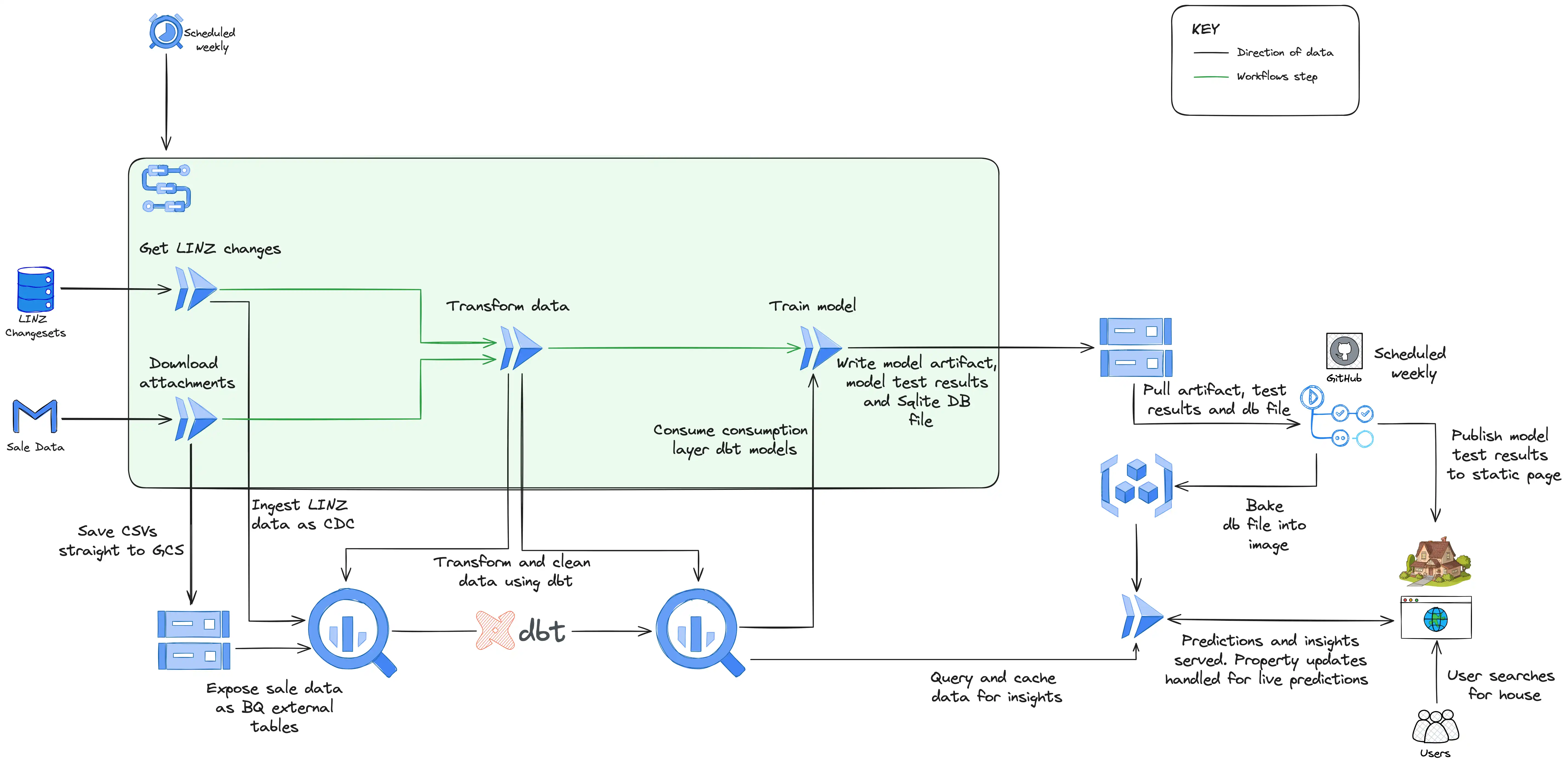
How House Pricer looks under the covers
The design above is how things hang together now, but it’s the result of several iterations and there’s certainly room for further iterating. We’ll get to that in a later section (to begin with it was just several Cloud Run jobs scheduled individually an hour apart!). At a high level it breaks down into three distinct sections:
- Data Ingestion - which involves getting the raw data into my data warehouse, BigQuery.
- Data Transformation and Model Training - which involves processing and cleaning the data so the model can use it to train
- Model Serving and the Website - which is finally presenting the predictions to users
Data Ingestion
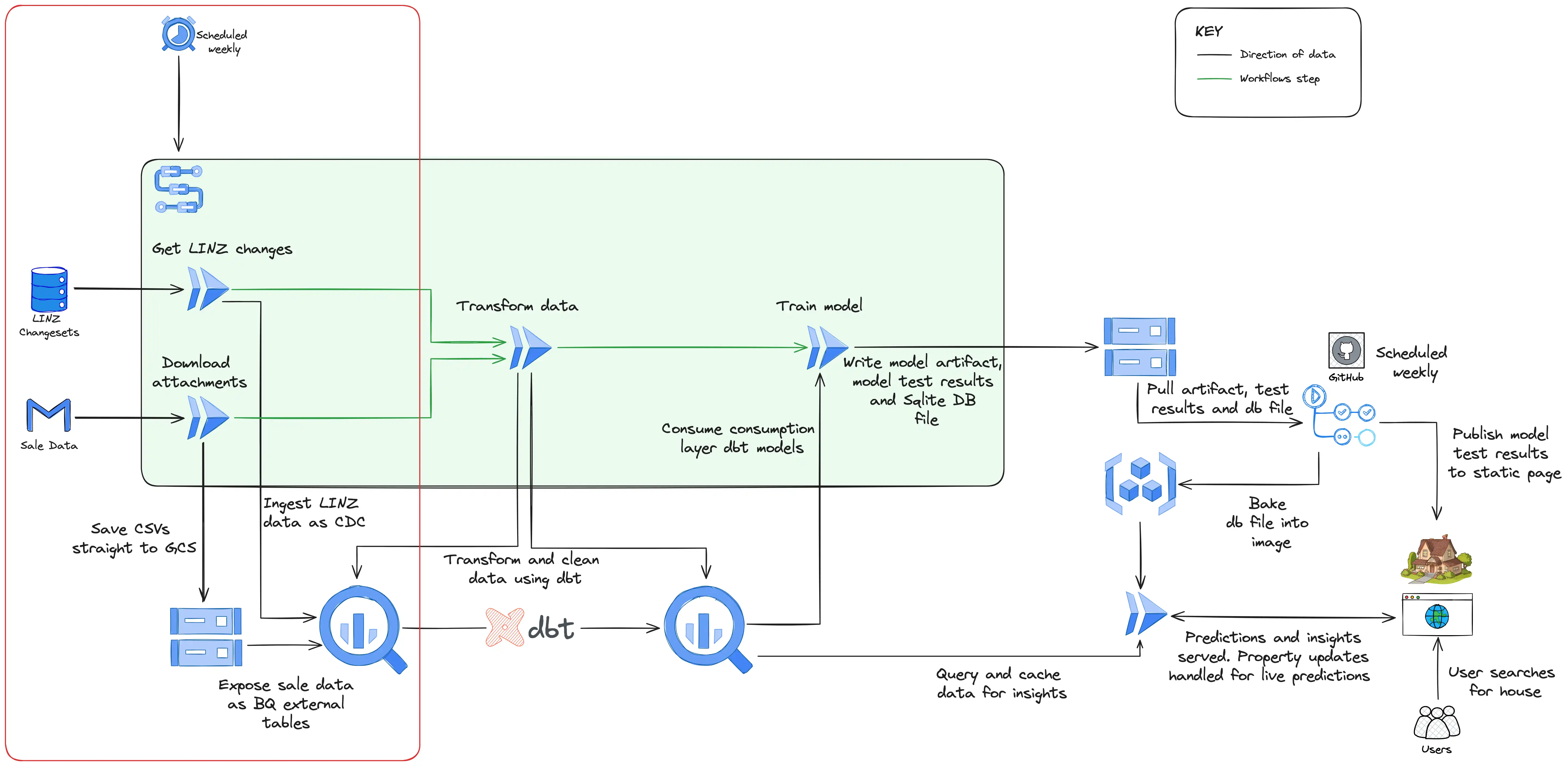
Data ingestion
Data arrives through two different methods: email attachment and API. Weekly on a Saturday, a workflow (using GCP Workflows) is kicked off by Cloud Scheduler which starts two Cloud Run jobs in parallel responsible for either downloading the sale data from Gmail or checking for changes to the LINZ data via their API.
In the case of the sale data, it’s uploaded directly to a Cloud Storage bucket which has a BigQuery external table exposing it and making it queryable downstream. I do this purely because it keeps the script to download from Gmail very simple - it’s just download the attachment and upload to Cloud Storage. BigQuery external tables also perform perfectly well for the volume of data I’m dealing with.
The acquisition of LINZ data is more elaborate (and interesting!). Their API returns a changeset containing rows with a column specifying it as either an insert, update, or delete. The Cloud Run job for this method streams this data directly into BigQuery using BigQuery’s support for Change Data Capture (CDC) which applies the updates automatically.
Data Transformation and Model Training
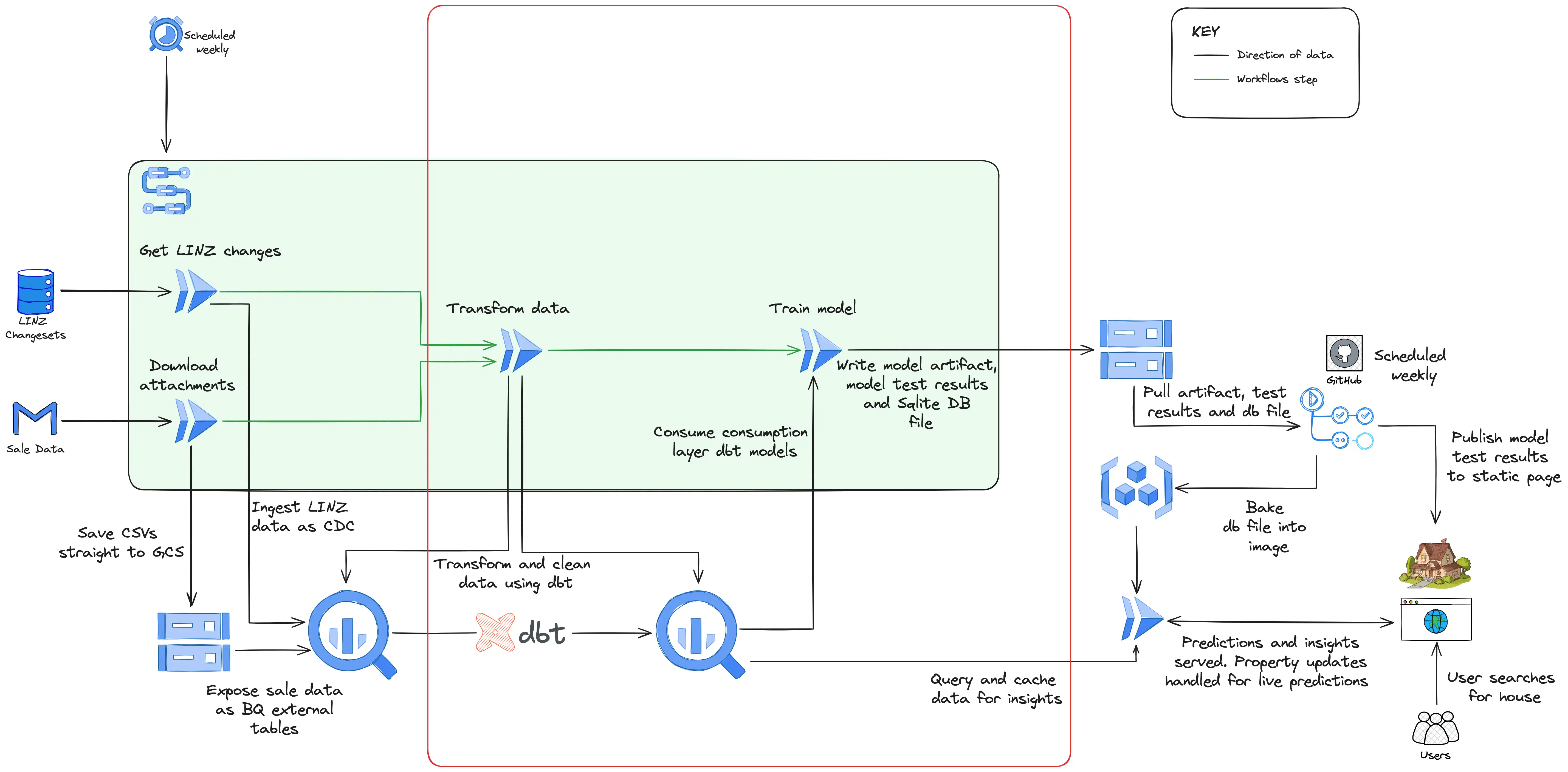
Data transformation
Once the data is in BigQuery, the next step is to massage it into a format that can be used by the model. This consists of removing outliers, joining datasets, and correcting errors where possible. The model expects input data which has correlations between the inputs and the output to be predicted (the sale price). That means it will perform well if there is a genuine connection between features fed into it such as location, size of the section, condition of the house. If these connections exist, with a complex enough model, it’ll find them. The balance is training a model that’s complex enough that it can find these relationships, but not so complex that it finds overly complex connections in the training data that aren’t representative of data it’s not yet seen (this is called over-fitting).
While developing the prototype model I created these transformations directly in my notebook using the Python library Pandas. While this is viable for exploratory work as little setup is required, when the transformations grow more complex and evolve (which they certainly have), it can become hard to manage. When it came to building the pipeline, I used a tool called dbt (intentionally lowercase) which is used for transforming data in a data warehouse such as BigQuery. Using dbt you create SQL models which can be easily version controlled and tested. The models which are materialised in BigQuery as views and tables, are laid out in an organised structure spanning from staging models which perform light cleaning of the source data (such as selecting columns and renaming) to intermediate models which combine other models and isolate complex operations, to finally the consumption models which are intended to be views or tables ready for use (in my case by the model training and analytics). In addition to this, dbt allows you to write automated tests against your SQL models and generate documentation and lineage graphs of the data.
Once dbt has run and generated or updated the consumption models with the latest sale and LINZ data, the model training job runs. To arrange this dependency and the dependency of the dbt run on the ingestion jobs from the previous section, I used the GCP service Workflows which allows you to define an order to tasks using YAML (if the ingestion step fails, there’s no point in running dbt or training the model as the data won’t have changed). The industry standard for orchestrating data pipelines like this is Airflow, but Airflow is a heavy and expensive tool which is certainly overkill for my use case (Google offers a managed Airflow service called Composer which starts at close to $1000 a month). Workflows is a very cheap alternative (I’m comfortably within the free tier) and provides the functionality I require which is to trigger jobs with dependencies.
Model Serving and the Website
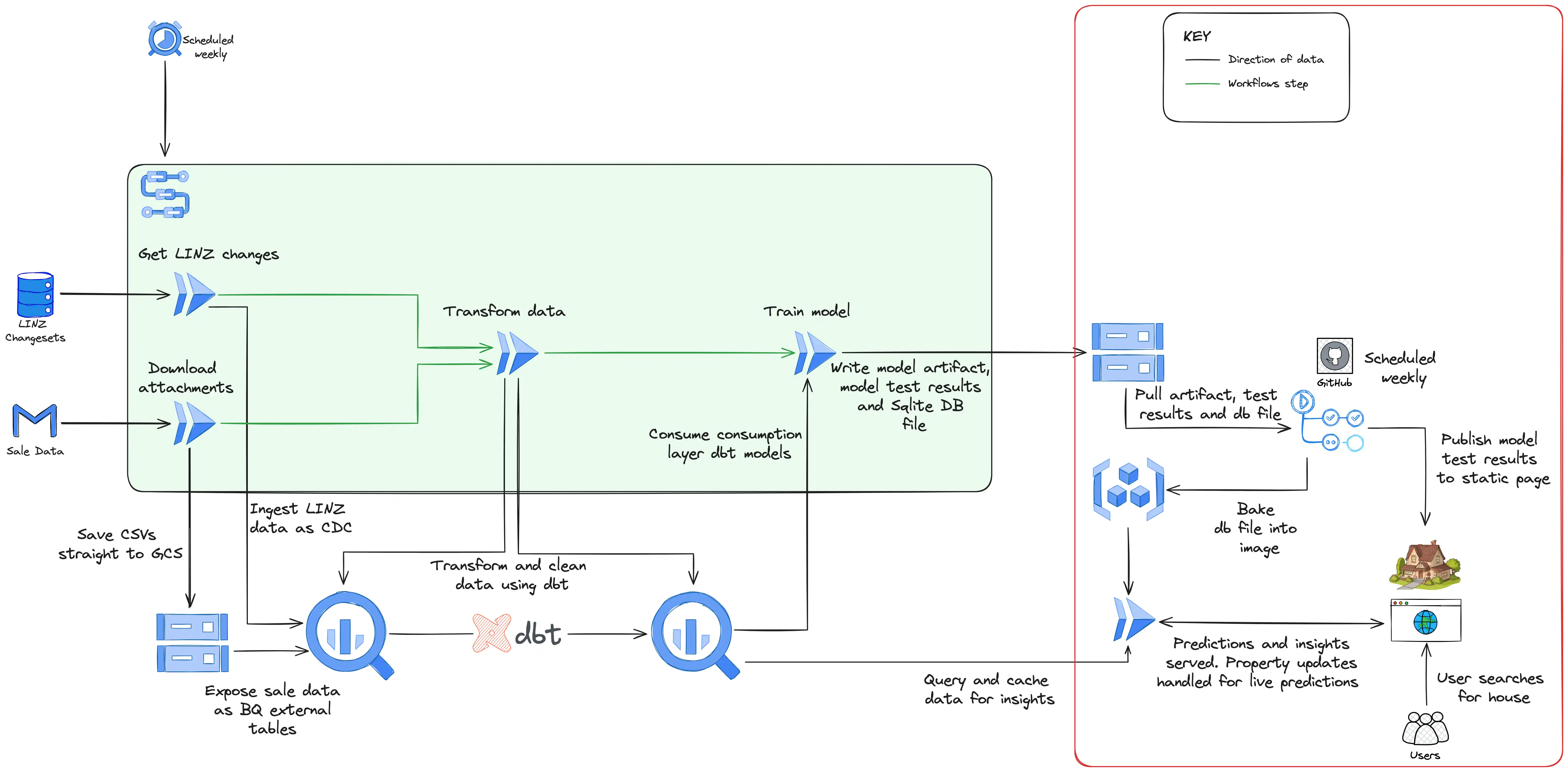
Model serving
This section of the project took by far the longest. My day job is data engineering and the concepts discussed already are things that I’m comfortable and experienced with. Designing the frontend in particular brought with it a challenge, but also an opportunity to develop skills.
In an early iteration of the model serving, I used Firestore to store and search the data and a Cloud Run service to act as the backend to the website. Firestore had the benefit that it was cheap (although still a few dollars a month), but the significant drawback was that it’s a document database and doesn’t support searching text natively which happened to be its most important job in this use case. To get around this limitation I had to implement complex logic in the model training job (which inserted into Firestore at the end) to index the data so that each address was split into overlapping trigrams, do the same in the Cloud Run service with the search text entered by the user on the website, and then match with a series of queries.
Given the pipeline runs weekly and so the data is only ever updated once a week, I decided to move to using an SQLite database running directly in the Cloud Run service. The model training job writes the results of the predictions along with the details of about 180k properties in Christchurch into an SQLite database and the database file is then uploaded to Cloud Storage. After this, a Github Action runs which pulls this database file and rebuilds the backend service’s docker image baking into it the database file, before deploying a new revision of the backend service with the updated SQLite database. I’m still yet to settle on this option as I suspect it won’t scale if I expand my website to the rest of New Zealand, but for now Cloud Run starts up very quickly, address searches are almost immediate, and it costs nothing at all to run. When the website hasn’t retrieved traffic for a certain time period, the Cloud Run service scales down to zero, and likewise when traffic increases, more instances are started to handle the increased load.
In addition to the database file being deployed in the Cloud Run service, several other artifacts are uploaded and deployed in this section of the pipeline. The results of the model tests (the model is trained on data up to 3 months ago, and then tested on the remaining 3 months of unseen data) are pushed to Cloud Storage and then pulled by Github Actions and deployed to the live website to show the accuracy of the model at this point in time. The model itself is also pushed to Cloud Storage, and then pulled by the Cloud Run service when a user uses the edit feature. This edit feature, which is live predictions made in real time, is not, to my knowledge, a feature supported by the other house estimate websites. Supporting live predictions on my House Pricer website opens the door to interesting applications such as “simulating” renovations and seeing how it’s expected to impact the price, or even taking an empty section and building a house on it (or several) and seeing the expected sale price.
3 Benefits and Future Improvements
The major benefit to this pipeline is that it costs mere cents to run each month and requires no human interaction. If House Pricer was to expand beyond Christchurch (property sale data is surprisingly expensive and tightly controlled), very little would need to change. BigQuery running the transformations is barely breaking a sweat with the current volume of data and it would likely still handle data for the entirety of New Zealand without leaving the free tier (1 TB of data processed a month is free).
The main area which could be improved in the future is the connection between Cloud Storage and Github Actions. Github Actions is used for the deployment of the Cloud Run service and the website purely because it’s familiar, but it does introduce a break in the ordered workflow. Once the model job runs, the Github Actions jobs run on a schedule set several hours after the model job is expected to finish. This means that if any of the Workflows section of the pipeline fails, the Github Actions jobs will still run. Instead I intend to make use of Cloud Build to handle the deployment at least of the Cloud Run service and trigger it off a Pubsub notification when the pipeline artifacts are uploaded to Cloud Storage (even better if Workflows supports triggering Cloud Build jobs).
Beyond this improvement however, the pipeline is in a production ready state and has been serving a steady stream of users over the last six months.
4 Conclusion
In this post we’ve seen how a machine learning pipeline which provides both batch and real-time predictions can be built on Google Cloud without barely leaving the free tier. Be sure to check out the finished product - a website called House Pricer here. With the advances of cloud computing and generous free tiers provided by the likes of Google Cloud, machine learning projects don’t have to be something restricted to the enterprise machine learning teams with huge budgets. Likewise, with the simplicity of services such as Cloud Run, BigQuery, and Workflows, machine learning ideas don’t need to become de-prioritised like the mostly finished DIY curtain rail installation at my house. The path to production has never been easier and as General George Patton Jr said “a good plan violently executed now is better than a perfect plan next week!”
If you have any questions or feedback, I’d love to hear so reach out on LinkedIn or email!